LASER
Introduction
LASER, which stands for Locating Ancestry using SEquencing Reads, is a C++ software package that can estimate individual ancestry directly from genome-wide shortgun sequencing reads without calling genotypes. The method relies on the availability of a set of reference individuals whose genome-wide SNP genotypes and ancestral information are known. We first construct a reference coordinate system by applying principal components analysis (PCA) to the genotype data of the reference individuals. Then, for each sequencing sample, use the genome-wide sequencing reads to place the sample into the reference PCA space. With an appropriate reference panel, the estimated coordinates of the sequencing samples identify their ancestral background and can be directly used to correct for population structure in association studies or to ensure adequate matching of cases and controls.
The goal of this wiki page is to help you get start using LASER, and we encourage you to read the manual for more details.
Download
To get a copy of the software and manual, go to the LASER Download page.
Workflow
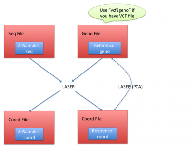
LASER generates the coordinates from both reference individuals and sequence samples. It requires essentially two input files:
- Seq file: a text file processed from BAM (alignment) files. (See Processing sequencing file for how to prepare seq file)
- Geno file: genotypes of reference individuals. (See Geno file to understand geno file format)
LASER typically output two coord files: (1) in reference individuals' coord file(Reference.coord), LASER outputs the reference coordinates in the PCA space; (2) in sequence samples' coord files(AllSamples.coord), LASER infers their ancestries by placing their ancestry coordinates onto reference samples' PCA space.
An example result of the coord file of sequence samples is shown below:
popID  indivID  L1    Ci        t         PC1       PC2
YRI    NA19238  1409  0.304122  0.98933   52.7634   -39.7924
CEU    NA12892  1552  0.330037  0.989709  9.82674   25.2898
CEU    NA12891  1609  0.362198  0.988082  0.439573  26.8872
CEU    NA12878  1579  0.334825  0.988677  8.83775   28.1342
YRI    NA19239  1558  0.34898   0.988302  53.9104   -39.1727
YRI    NA19240  1735  0.404142  0.990264  59.8379   -45.2765
In the header line, popID means "population ID", indivID means "individual ID", L1 means number of loci that has been covered by at least one read, Ci means "average coverage", t means Procrustes similarity. PC1, PC2 means coordinates of the first and second principal components.
Tutorial
In this tutorial, we will show you how to prepare data and run LASER.
Process sequencing file (BAM)
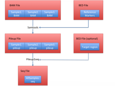
We illustrate how to obtain .seq file from BAM files in this section. In this example, we use HGDP data set as reference, which contains 938 individuals and 632,958 markers.
1. Obtain pileup files from BAM files
We use samtools to extract the sequence bases overlapping the 632,958 reference markers:
samtools mpileup -q 30 -Q 20 -f ../../LASER-resource/reference/hs37d5.fa -l HGDP_938.bed exampleBAM/NA12878.chrom22.recal.bam > NA12878.chrom22.pileup
2. Obtain a seq file from pileup files.
To convert pileup files into a single seq file before running LASER, we first generate a site file:
cat ../resource/HGDP/HGDP_938.site |awk '{if (NR > 1) {print $1, $2-1, $2;}}' > HGDP_938.bed
Then use this site file and all generated pileup files from step 1 to generate a seq file:
python pileup2seq.py -m ../resource/HGDP/HGDP_938.site -o test NA12878.chrom22.pileup
Estimate ancestries of sequence samples
The easiest way to perform LASER using its exemplar data is:
./laser -s pileup2seq/test.seq -g resource/HGDP/HGDP_938.geno -c resource/HGDP/HGDP_938.RefPC.coord -o test -k 2
Upon successful calculation, you will find a result file "test.SeqPC.coord".
File format
Geno file
In our resource folder, we provide an example geno file for the HGDP data set (resource/HGDP/HGDP_938.geno):
Brahui	HGDP00001	1	2	1	1	0	2	0	2	1	2	2	2	1	1	2	1	0
Brahui	HGDP00003	0	0	2	0	0	2	0	2	0	2	2	2	2	0	2	2	0
Brahui	HGDP00005	0	2	2	0	0	1	0	2	1	2	2	2	2	1	2	2	1
Brahui	HGDP00007	0	2	2	0	0	2	0	2	0	2	2	2	1	1	2	2	1
Brahui	HGDP00009	0	1	0	1	0	2	0	2	0	2	2	2	2	0	2	2	0
Brahui	HGDP00011	1	1	2	1	1	2	1	1	1	2	2	2	1	1	2	2	0
Brahui	HGDP00013	1	2	2	1	1	2	1	2	0	2	2	2	2	0	2	2	0
Brahui	HGDP00015	1	1	2	0	0	2	0	2	0	2	2	2	2	0	2	2	0
Brahui	HGDP00017	1	1	2	0	0	1	0	0	0	2	0	1	1	2	2	2	0
Brahui	HGDP00019	0	2	2	0	0	1	0	1	0	2	1	2	2	1	2	2	0
The first and second columns represent the population id and individual id. From the third column, each number represents a genotype. In this geno file, we have 632,960 columns which contains 632,958 markers from column 3 to the last column.
Seq file
Seq file is generated from pileup files. It contains sequencing information and organize it in a LASER readable format. The first two columns represent population id and individual id. Subsequent columns are total read depths and reference base counts. For example, column 3 and 4 are 0, 0 in the following example. That means at first marker, the sequence read depth is 0 and thus none of the reads has reference base. We enforce tab delimiters between markers and space delimiters between each read depths and reference base counts. On line of seq file looks like below:
NA12878.chrom22 NA12878.chrom22 0 0 0 0 0 0 0 0 0
Pileup file
Pileup file are generate using samtools. An example pileup file is shown below:
22	17094749	A	1	c	D
22	17202602	T	1	.	D
22	17411899	A	1	.	C
22	17450515	G	2	.,	9<
22	17452966	T	1	c	5
22	17470779	C	1	,	A
22	17492203	G	1	,	B
22	17504945	C	3	,..	BCA
22	17529814	T	3	..,	CCC
The columns are chromosome, position (1-based), reference base, depth, bases and base qualities.
BED file
BED file represents genomic regions and it follows UCSC conventions:
1 752565 752566
1 768447 768448
1 1005805 1005806
1 1018703 1018704
1 1021414 1021415
The columns are: chromosome, start position (0-based) and end position (1-based).
Coord file
Coord files represent the ancestries of both reference samples and sequence samples. An example coord file looks like below:
popID  indivID  L1    Ci        t         PC1       PC2
YRI    NA19238  1409  0.304122  0.98933   52.7634   -39.7924
CEU    NA12892  1552  0.330037  0.989709  9.82674   25.2898
CEU    NA12891  1609  0.362198  0.988082  0.439573  26.8872
CEU    NA12878  1579  0.334825  0.988677  8.83775   28.1342
YRI    NA19239  1558  0.34898   0.988302  53.9104   -39.1727
YRI    NA19240  1735  0.404142  0.990264  59.8379   -45.2765
The columns are: popID means "population ID", indivID means "individual ID", L1 means number of loci has been covered, Ci means "average coverage", t means Procrustes similarity. PC1, PC2 means coordinates of first and second principal components. You may notice L1, Ci, and t are omitted in the coord files of reference samples. The reason is that reference samples use genotypes and do not have coverage information.
Site file
Site file is equivalent to BED file and it is used here to represent marker positions. An example site file looks like below:
CHR  POS      ID          REF  ALT
1    752566   rs3094315   G    A
1    768448   rs12562034  G    A
1    1005806  rs3934834   C    T
1    1018704  rs9442372   A    G
1    1021415  rs3737728   A    G
The site file has header line, and it contains chromosome, position(1-based), id (usually marker name), ref (reference allele) and alt (alternative allele).
Advanced options
LASER has advanced options including (1) parallel computing; (2) increase ancestry inference accuracy using repeated runs; (3) generate PCA coordiates using genotypes. See LASER Manual for detailed information.
Contact
Comments on this wiki page or questions related to preparing input files for LASER can be sent to Xiaowei Zhan. Comments on the LASER software or the user's manual can be sent to Chaolong Wang. This project was directed by Gonçalo Abecasis and Sebastian Zöllner at the University of Michigan.

