LocusZoom Standalone

This page contains information regarding a version of LocusZoom that may be downloaded for personal use. For more information on LocusZoom, see this page.

Requirements

The following software is required:

• Python 2.6 (do not download the 3.0 branch!)
• R 2.10+
• new_fugue, a program for computing LD, written by Goncalo Abecasis.

Currently only Unix/Linux is supported, though Mac OS X should be supported in a future release.

Synopsis

A quick example

First, change directory into examples/. Then, run the following command:

./run_example.py

This script runs the following command for you:

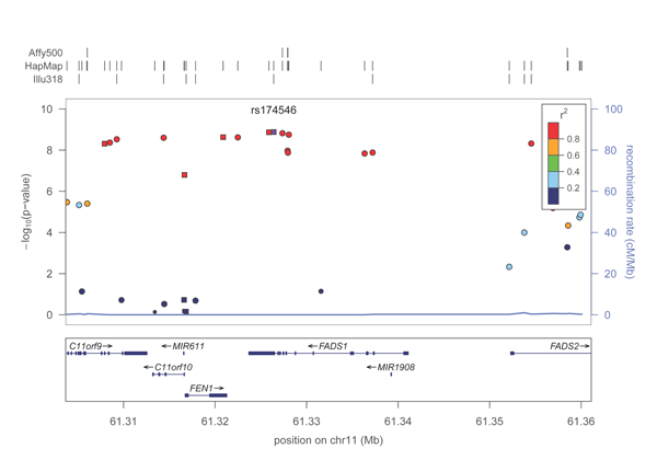
../bin/locuszoom --metal Kathiresan_2009_HDL.txt --refgene FADS1

A PDF plot of the FADS1 locus will be created in the directory. It should look roughly like this:

Voila, your first region plot!

Installation

Step 1: Install Python

You will need to install Python on your system if it is not already. Head over to www.python.org to download it. Note that you will want to make sure to download the latest from the 2.x branch, and not the 3.0 one.

Step 2: Install R

R is also required for generating the plots. You can download R at www.r-project.org. Version 2.10 or greater is required.

Step 3: Install new_fugue

New_fugue is a program that calculates linkage disequilibrium measures from genotype files. While installing new_fugue is optional, we highly recommend it as it makes the process of generating plots much easier. If you opt to skip installing new_fugue, you will need to provide your own computed LD files for each region that you want to plot.

New_fugue can be downloaded from here.

Once downloaded, extract the tar file using:

 tar zxf /path/to/new_fugue.tar.gz

Change into the generic-new_fugue directory that is created, and run:

 make install 

Step 4: Install LocusZoom

LocusZoom is provided as a tar archive which contains the following:

• the LocusZoom python application
• the R script used for generating plots
• genotype files (used for computing LD) from hapmap and 1000G (build hg18 only)
• a SQLite database file containing tables describing SNP positions, SNP annotations, gene and exon locations, and recombination rates (build hg18 only)

Simply unpack the tar to your directory of choice by doing the following:

cd <directory where you want to place locuszoom> 
tar zxf /path/to/locuszoom.tgz 

The tar archive will extract into the following directory structure:

• locuszoom/
  • bin/
    • locuszoom (this is the locuszoom "executable")
    • locuszoom.R (the R script which is used by locuszoom for creating the plots)
  • conf/ (configuration file located here)
  • data/
    • database/ (SQLite file located here)
    • hapmap/ (hapmap genotype files)
    • 1000G/ (1000G genotype files)
  • src/ (source code for locuszoom)

It is important that this directory structure remain intact. To make launching locusoom easier, you could create a link to it from /usr/local/bin, for example:

ln -s bin/locuszoom /usr/local/bin/locuszoom

Input

Association results file ("metal" file)

The main input to LocusZoom is a file containing results from an association scan or meta-analysis. The file must have 2 things: markers (SNPs), and p-values. The file should look something like this:

MarkerName	P-value
rs1	0.423
rs2	1.23e-04
rs3	9.4e-390

The file should be tab-delimited, though this can be changed using the --delim option.

This file should be passed to locuszoom using the --metal option.

If your marker and p-value column names are not "MarkerName" and "P-value", you may set them with --markercol and --pvalcol options.

Region

You can specify the region to plot in any one of the following ways:

• A reference SNP and flanking region

 --refsnp <your snp> --flank 500kb 

• A reference SNP and chromosome/start/stop specification

 --refsnp <your snp> --chr # --start <base position> --end <base position> 

• A gene and flanking region

 --refgene <your gene> --flank 250kb 

The flank is computed as +/- from the transcription start/end of the gene. From this region, LocusZoom will find the SNP with the most significant p-value, and use this as the reference SNP.

• A gene and chromosome/start/stop specification

 --refgene <your gene> --chr # --start <base position> --end <base position> 

This method is similar to the above, except that an exact region is specified. The SNP with the most significant p-value in this region will be used.

• A chromosome/start/stop specification

 --chr # --start <base position> --end <base position> 

Once again, the SNP with the most significant p-value will be used in this region.

Output

LocusZoom will produce a directory for each plot that contains the plot itself, along with a number of temporary files containing information on your particular region. The plot will be a PDF, named with the chr#:start-stop that was plotted.

If you only want the PDF itself, and don't want the other files, you can use the --plotonly option.

Each directory (or PDF, in the case of --plotonly) will have the date included to avoid collisions with previous plots - this behavior can be disabled using --no-date.

You can further customize the directory/PDF names that are created by using the --prefix <name> option. This will append a text string at the beginning of each directory/PDF that is created.