SeqShop: Variant Calling and Filtering for INDELs Practical, June 2014
Goals of This Session
- What we want to learn
- How to generate variant calls for INDELs from BAMs
- How to examine the variants at particular genomic positions
- How to evaluate the quality of INDEL calls
Setup in person at the SeqShop Workshop
This section is specifically for the SeqShop Workshop computers.
If you are not running during the SeqShop Workshop, please skip this section.
Login to the seqshop-server Linux Machine
This section will appear redundantly in each session. If you are already logged in or know how to log in to the server, please skip this section
- Login to the windows machine
- The username/password for the Windows machine should be written on the right-hand monitor
- Start xming so you can open external windows on our Linux machine
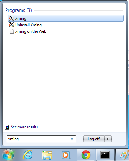
- Start->Enter "Xming" in the search and select "Xming" from the program list
- Nothing will happen, but Xming was started.
- Open putty
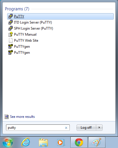
- Start->Enter "putty" in the search and select "PuTTY" from the program list
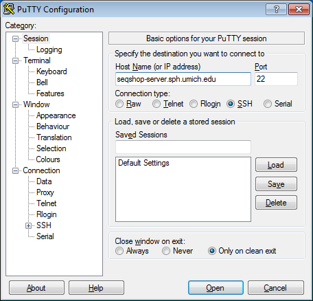
- Configure PuTTY in the PuTTY Configuration window
- Host Name:
seqshop-server.sph.umich.edu - Setup to allow you to open external windows:
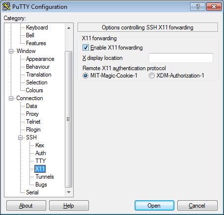
- In the left pannel: Connection->SSH->X11
- Add a check mark in the box next to
Enable X11 forwarding - Click
Open - If it prompts about a key, click
OK - Enter your provided username & password as provided
You should now be logged into a terminal on the seqshop-server and be able to access the test files.
- If you need another terminal, repeat from step 3.
Login to the seqshop Machine
So you can each run multiple jobs at once, we will have you run on 4 different machines within our seqshop setup.
- You can only access these machines after logging onto seqshop-server
3 users logon to:
ssh -X seqshop1
3 users logon to:
ssh -X seqshop2
2 users logon to:
ssh -X seqshop3
2 users logon to:
ssh -X seqshop4
Setup your run environment
This is the same setup you did for the previous tutorial, but you need to redo it each time you log in.
This will setup some environment variables to point you to
- GotCloud program
- Tutorial input files
- Setup an output directory
- It will leave your output directory from the previous tutorial in tact.
source /home/mktrost/seqshop/setup.txt
- You won't see any output after running
source- It silently sets up your environment
- If you want to view the detail of the setup, type
less /home/mktrost/seqshop/setup.txt
and press 'q' to finish.
Setup when running on your own outside of the SeqShop Workshop
This section is specifically for running on your own outside of the SeqShop Workshop.
If you are running during the SeqShop Workshop, please skip this section.
This tutorial builds on the alignment tutorial, if you have not already, please first run that tutorial: Alignment Tutorial
It also uses the bam.index file created in the SnpCall Tutorial. If you have not yet run that tutorial, please follow the directions at: GotCloud BAM Index File
Setup your run environment
Environment variables will be used throughout the tutorial.
We recommend that you setup these variables so you won't have to modify every command in the tutorial.
- Point to where you installed GotCloud
- Point to where you installed the seqshop files
- Point to where you want the output to go
- Using bash (replace the paths below with the appropriate paths):
export GC=~/seqshop/gotcloud
export SS=~/seqshop/example
export OUT=~/seqshop/output
- Using tcsh (replace the paths below with the appropriate paths):
setenv GC ~/seqshop/gotcloud
setenv SS ~/seqshop/example
setenv OUT ~/seqshop/output
Examining GotCloud Indel Input files
The GotCloud Indel caller takes the same inputs as GotCloud snpcall.
- BAMs->INDELs rather than BAMs->SNPs
If you want a reminder, of what they look like, here is a link to the previous tutorial : GotCloud SnpCall Input Files
Running GotCloud Indel
${GC}/gotcloud indel --conf ${SS}/gotcloud.conf --numjobs 2 --region 22:36000000-37000000 --base_prefix ${SS} --outdir ${OUT}
${GC}/gotcloudruns GotCloudindeltells GotCloud you want to run the indel calling pipeline.--conftells GotCloud the name of the configuration file to use.- The configuration for this test was downloaded with the seqshop input files.
- --numjobs tells GotCloud how many jobs to run in parallel
- Depends on your system
- --region 22:36000000-37000000
- The sample files are just a small region of chromosome 22, so to save time, we tell GotCloud to ignore the other regions
--base_prefixtells GotCloud the prefix to append to relative paths.- The Configuration file cannot read environment variables, so we need to tell GotCloud the path to the input files, ${SS}
- Alternatively, gotcloud.conf could be updated to specify the full paths
--out_dirtells GotCloud where to write the output.- This could be specified in gotcloud.conf, but to allow you to use the ${OUT} to change the output location, it is specified on the command-line
This should take about 4-5 minutes to run.
- It should end with a line like:
Commands finished in 289 secs with no errors reported
If you cancelled GotCloud part way through, just rerun your GotCloud command and it will pick up where it left off.
Examining GotCloud indel Ouptut
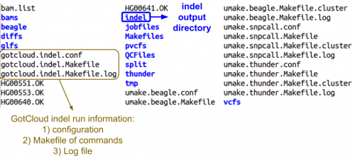
Let's look at the output directory:
ls ${OUT}
- Do you see any new files or directories?
Let's look at the final directory:
ls ${OUT}/final
- Can you identify the final indel VCF?
Did I find interesting variants?
The region we selected contains APOL1 gene, which is known to play an important role in kidney diseases such as nephrotic syndrome. There are two risk alleles in protein-coding region of this gene.
- g1 allele is non-synonymous risk allele,
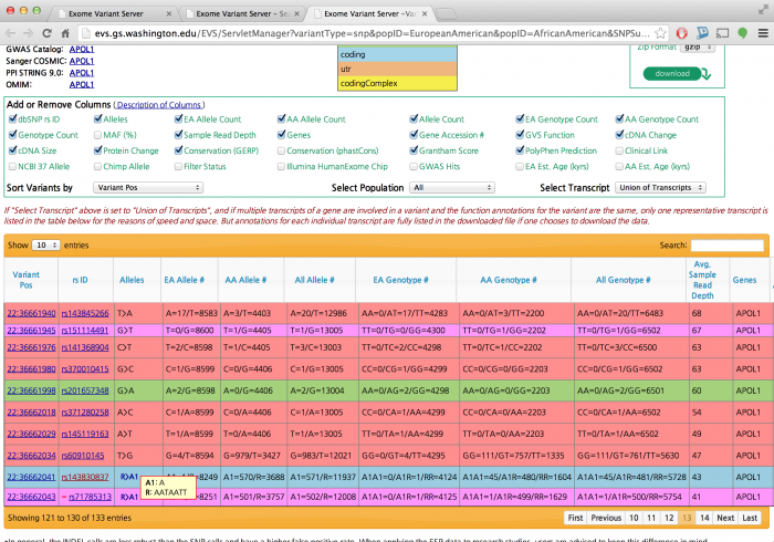
rs73885139located at position22:36661906increases the risk of nephrotic syndrome by >2-folds. We looked at this variant in the morning. - g2 allele is an 6-base deletion (in-frame indel), located the end of the APOL1 gene. It has smaller than g1 but still large effect size (>1.5 fold). Let's see if we have found the variant.
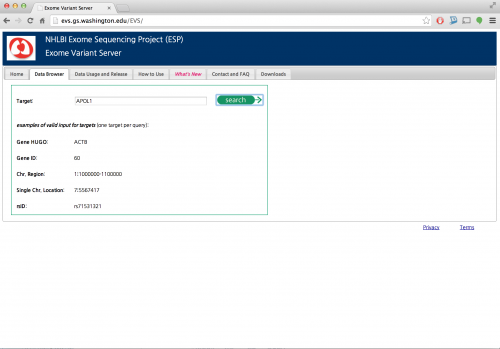
First, look up the indels by navigating exome variant server.
Focusing on APOL1 gene,
You will be able to find the in-frame indel near the end of the gene
Let's see if we found the indel
${GC}/bin/tabix ${OUT}/final/all.genotypes.vcf.gz 22:36662041 | head -1
Did you see a variant at the position?
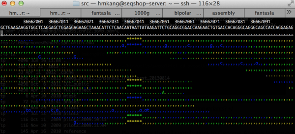
Let's check the sequence data to confirm that the variant really exists
${GC}/bin/samtools tview ${SS}/bams/HG01101.recal.bam ${SS}/ref22/human.g1k.v37.chr22.fa
- Type 'g' to go to a specific position
- Type 22:36662041 to move to the position
- Press arrows to move between positions
- Press 'b' if you want to color by base quality
- Press '?' for more help
Details of the output file
Looking at the INDEL Variant Call File (VCF)
We will use Vt or tabix to look at the INDEL VCF file.
Header
First, let's look at the header:
${GC}/bin/tabix -H ${OUT}/final/all.genotypes.vcf.gz
The header is as follows:
 ##fileformat=VCFv4.2
 ##FILTER=<ID=PASS,Description="All filters passed">
 ##contig=<ID=22,length=51304566>
 ##FORMAT=<ID=GT,Number=1,Type=String,Description="Genotype">
 ##FORMAT=<ID=PL,Number=G,Type=Integer,Description="Normalized, Phred-scaled likelihoods for genotypes">
 ##FORMAT=<ID=DP,Number=1,Type=Integer,Description="Depth">
 ##FORMAT=<ID=AD,Number=3,Type=Integer,Description="Allele Depth">
 ##FORMAT=<ID=GQ,Number=1,Type=Integer,Description="Genotype Quality">
 ##INFO=<ID=AC,Number=A,Type=Integer,Description="Alternate Allele Counts">
 ##INFO=<ID=AN,Number=1,Type=Integer,Description="Total Number Allele Counts">
 ##INFO=<ID=NS,Number=1,Type=Integer,Description="Number of Samples With Data">
 ##INFO=<ID=AF,Number=A,Type=Float,Description="Alternate Allele Frequency">
 ##INFO=<ID=GC,Number=G,Type=Integer,Description="Genotype Counts">
 ##INFO=<ID=GN,Number=1,Type=Integer,Description="Total Number of Genotypes Counts">
 ##INFO=<ID=GF,Number=G,Type=Float,Description="Genotype Frequency">
 ##INFO=<ID=HWEAF,Number=A,Type=Float,Description="Genotype likelihood based MLE Allele Frequency assuming HWE">
 ##INFO=<ID=HWEGF,Number=G,Type=Float,Description="Genotype likelihood based MLE Genotype Frequency assuming HWE">
 ##INFO=<ID=MLEAF,Number=A,Type=Float,Description="Genotype likelihood based MLE Allele Frequency">
 ##INFO=<ID=MLEGF,Number=G,Type=Float,Description="Genotype likelihood based MLE Genotype Frequency">
 ##INFO=<ID=HWE_LLR,Number=1,Type=Float,Description="Genotype likelihood based Hardy Weinberg ln(Likelihood Ratio)">
 ##INFO=<ID=HWE_LPVAL,Number=1,Type=Float,Description="Genotype likelihood based Hardy Weinberg Likelihood Ratio Test Statistic ln(p-value)">
 ##INFO=<ID=HWE_DF,Number=1,Type=Integer,Description="Degrees of freedom for Genotype likelihood based Hardy Weinberg Likelihood Ratio Test Statistic">
 ##INFO=<ID=FIC,Number=1,Type=Float,Description="Genotype likelihood based Inbreeding Coefficient">
 ##INFO=<ID=AB,Number=1,Type=Float,Description="Genotype likelihood based Allele Balance">
 ##FILTER=<ID=PASS,Description="Temporary pass">
 ##FILTER=<ID=overlap,Description="Overlapping variant">
 #CHROM	POS	ID	REF	ALT	QUAL	FILTER	INFO	FORMAT	HG00551	HG00553	HG00554	HG00637	HG00638	HG00640	HG00641	HG00734	HG00736	HG00737	HG00739	HG00740	HG01047	HG01049	HG01051	HG01052	HG01054	HG01055	HG01060	HG01061	HG01066	HG01067	HG01069	HG01070	HG01072	HG01073	HG01075	HG01079	HG01080	HG01082	HG01083	HG01094	HG01097	HG01098	HG01101	HG01102	HG01107	HG01108	HG01110	HG01111	HG01167	HG01168	HG01170	HG01171	HG01173	HG01174	HG01176	HG01177	HG01182	HG01183	HG01187	HG01188	HG01190	HG01191	HG01197	HG01198	HG01204	HG01205	HG01241	HG01242	HG01247	HG01248
Using Vt, we can see the same output
${GC}/bin/vt view -H ${OUT}/final/all.genotypes.vcf.gz
Records
To view a specific region of records (such as APOL1 g2 allele)
${GC}/bin/tabix ${OUT}/final/all.genotypes.vcf.gz 22:36662041-36662041
The columns are CHROM, POS, ID, REF, ALT, QUAL, FILTER, INFO, FORMAT, Genotype fields denoted by the sample name.
22	36662041	.	AATAATT	A	756	PASS AC=2;AN=114;AF=0.0175439;GC=55,2,0;GN=57;
                         GF=0.964912,0.0350877,0;NS=57;
                         HWEAF=0.019571;HWEGF=0.961242,0.038376,0.000383024;
                         MLEAF=0.0196187;MLEGF=0.960762,0.0392374,2.11537e-15;
                         HWE_LLR=-0.0222464;HWE_LPVAL=-0.182794;HWE_DF=1;
                         FIC=-0.00372601;AB=0.384578
                      GT:PL:DP:AD:GQ	0/0:0,9,158:3:3,0,0:10	0/0:0,18,281:6:6,0,0:18
Here is a description of the record's fields.
 22             : chromosome
 36662041       : genome position
 .              : this is the ID field that is left blank.
 AATAATT        : the reference sequence that is replaced by the alternative sequence below.
 A              : so this is basically a deletion of GT
 756            : QUAL field denoting validity of this variant, higher the better.
 PASS           : a passed variant.
 INFO           : fields containing information about the variant.
 FORMAT         : format field labels for the genotype columns.
 0/0:0,9,158:3:3,0,0:10 :  genotype information.
You can obtain the same output by using the following command
${GC}/bin/vt view -i 22:36990878-36990879 ${OUT}/final/all.genotypes.vcf.gz
- -i specifies the region
- You can leave it out and look at all the records
INFO field
The key information fields are as follows:
 AC=2                 : alternate allele count
 AN=114               : total number of alleles
 AF=0.017             : allele frequency based on AC/AN
 GC=55,2,0            : genotype counts for 0/0, 0/1, 1/1
 GF=0.55,0.34,0.10    : genotype frequencies based on GC
 NS=57                : no. of samples
 HWEAF=0.28           : genotype likelihood based estimation of the allele frequency assuming Hardy Weinberg equilibrium
 HWEGF=0.52,0.40,0.08 : genotype frequency derived from HWEAF
 HWE_LPVAL=-1.08      : log p value of HWE test
 FIC=-0.07            : genotype likelihood based inbreeding coefficient
 AB=0.61              : genotype likelihood based allele balance
GENOTYPE field
The genotype fields are described as follows:
 0/0      : homozygous reference chosen based on PL
 0,9,158  : PHRED scaled genotype likelihoods
 3        : no. of reads covering this variant
 3,0,0    : allele depth
            counts of reads supporting the reference allele,
            the alternative allele and neither alleles respectively.
            The last category might be due to insufficient
            coverage of the read over the locus
            or simply an allele that is not accounted for.
 10       : genotype quality
INDEL Analysis
The following section details some simple analyses we can perform.
Summary
First you want to know what is in the vcf file.
${GC}/bin/vt peek ${OUT}/final/all.genotypes.vcf.gz
 stats: no. of samples                     :         62
        no. of chromosomes                 :          1

        no. Indels                         :        720
            2 alleles (ins/del)            :             720 (0.84) [328/392] #(insertion deletion ratio) [#insertions, #deletions]
            >=3 alleles (ins/del)          :               0 (-nan) [0/0]

        no. of observed variants           :        720
- Our VCF only contains only biallelic INDELs so there are lots of
0 (-nan) [0/0]values in the output.vtcan be used to analyze VCFs with more variants than just INDELs.
The variants have filter labels. PASS meaning a passed variant and overlap, meaning that the variants are overlapping with another variant, implying multiallelicity.
We can count the number of variants with different filters with the following commands.
${GC}/bin/vt peek ${OUT}/final/all.genotypes.vcf.gz -f "FILTER.PASS"
 stats: no. of samples                     :         62
        no. of chromosomes                 :          1

        no. Indels                         :        584
            2 alleles (ins/del)            :             584 (0.69) [239/345]
            >=3 alleles (ins/del)          :               0 (-nan) [0/0]
${GC}/bin/vt peek ${OUT}/final/all.genotypes.vcf.gz -f "FILTER.overlap"
 stats: no. of samples                     :         62
        no. of chromosomes                 :          1

        no. Indels                         :        136
            2 alleles (ins/del)            :             136 (1.89) [89/47]  #notice the difference in insertion deletion ratios
            >=3 alleles (ins/del)          :               0 (-nan) [0/0]
 #passed singletons only
 ${GC}/bin/vt peek ${OUT}/final/all.genotypes.vcf.gz -f "FILTER.PASS&&INFO.AC==1"

 #passed indels of length 1 only
 ${GC}/bin/vt peek ${OUT}/final/all.genotypes.vcf.gz -f "FILTER.PASS&&LEN==1"

 #passed indels of length >4
 ${GC}/bin/vt peek ${OUT}/final/all.genotypes.vcf.gz -f "FILTER.PASS&&LEN>4"

 #passed singletons of length 4 or insertions of length 3
 ${GC}/bin/vt peek ${OUT}/final/all.genotypes.vcf.gz -f "FILTER.PASS&&(LEN==4||DLEN==3)"
Comparison with other data sets
It is usually useful to examine the call sets against known data sets for the passed variants.
In order to do this, you need to update indel.reference.txt to point to the reference files.
cp ${SS}/ref22/indel.reference.txt ${OUT}/indel.reference.txt
Edit indel.reference.txt and specify the correct path to ${SS}
nedit ${OUT}/indel.reference.txt
- Replace all occurrences of
usernamewith your username (or the correct path to your seqshop example directory).
${GC}/bin/vt profile_indels -g ${OUT}/indel.reference.txt -r ${SS}/ref22/human.g1k.v37.chr22.fa ${OUT}/final/all.genotypes.vcf.gz -i 22:36000000-37000000 -f "PASS"
 data set
   No Indels         :        613 [0.72]    #613 passed variants with an insertion deletion ratio of 0.72
      FS/NFS         :       0.50 (2/2)     #frame shift / non frameshift indels proportion, the bracket gives the counts of the frame shift and non frameshift indels
      Low complexity :       0.46 (283/613) #fraction of indels in low complexity region, the bracket gives the counts of the indels

 1000G  #1000 Genomes Phase 1 data set
   A-B        371 [0.76] #variants found in call set only, square brackets contain insertion deletion ratio
   A&B        242 [0.66] #variants found in both data sets
   B-A        276 [0.89] #variants found in 1000G phase 1 data set only
   Precision    39.5%    #39.5% of the call set are previously known, so 60.5% are novel variants.
   Sensitivity  46.7%    #sensitivity of variant calling, 46,7% of known variants from 1000 Genomes were rediscovered

 mills  #The gold standard Mills et al. indel set
   A-B        542 [0.68]
   A&B         71 [1.03]
   B-A         31 [1.07]
   Precision    11.6%
   Sensitivity  69.6%

 dbsnp  #Indels from dbSNP
   A-B        405 [0.68]
   A&B        208 [0.79]
   B-A        494 [2.03]
   Precision    33.9%
   Sensitivity  29.6%
Ins/Del ratios: Reference alignment based methods tend to be biased towards the detection of deletions. This provides a useful measure for discovery Indel sets to show the varying degree of biasness. It also appears that as coverage increases, the ins/del ratio tends to 1.
Coding region analysis: Coding region Indels may be categorised as Frame shift Indels and Non frameshift Indels. A lower proportion of Frameshift Indels may indicate a better quality data set but this depends also on the individuals sequenced.
Complexity region analysis: Indels in regions marked by DUST - a low complexity region masker used in the NCBI pipeline.
Overlap analysis: overlap analysis with other data sets is an indicator of sensitivity.
- 1000G: contains Indels from 1000 Genomes, represent a wide spectrum of variants from many different populations. Variants here have an allele frequency above 0.005.
- Mills: contains doublehit common indels from the Mills. et al paper and is a relatively good measure of sensitivity for common variants. Because not all Indels in this set is expected to be present in your sample, this actually gives you an underestimate of sensitivity.
- dbsnp: contains Indels submitted from everywhere, I am not sure what does this represent exactly. But assuming most are real, then precision is a useful estimated quantity from this reference data set.
We perform the same analysis for the failed variants again, the relatively low overlap with known data sets imply a reasonable tradeoff in sensitivity and specificity.
${GC}/bin/vt profile_indels -g ${OUT}/indel.reference.txt -r ${SS}/ref22/human.g1k.v37.chr22.fa ${OUT}/final/all.genotypes.vcf.gz -i 22:36000000-37000000 -f "~PASS"
 data set
   No Indels         :        107 [2.06]
      FS/NFS         :       -nan (0/0)
      Low complexity :       0.79 (85/107)

 1000G
   A-B        107 [2.06]
   A&B          0 [-nan]
   B-A        518 [0.77]
   Precision     0.0%
   Sensitivity   0.0%

 mills
   A-B        105 [2.09]
   A&B          2 [1.00]
   B-A        100 [1.04]
   Precision     1.9%
   Sensitivity   2.0%

 dbsnp
   A-B        102 [2.00]
   A&B          5 [4.00]
   B-A        697 [1.51]
   Precision     4.7%
   Sensitivity   0.7%
This analysis supports filters too.
Normalization
A slight digression here, when analyzing indels, it is important to normalize it. While it is a simple concept, it is hardly standardized. The call set here had already been normalized but we feel that this is an important concept so we discuss this a bit here.
Indel representation is not unique, you should normalize them and remove duplicates.
  Variant normalization is implemented in vt and this page explains the algorithm
  and also provides a simple proof of correctness - Variant Normalization
The following table shows the number of variants that had to be normalized and the corresponding type of normalization performed and the ensuing number of duplicate variants found for some of the 1000 Genomes Trio High Coverage call sets. Although left alignment seems to be a trivial concept, it is easily overlooked and remain a common mistake.
| Dataset | Haplotyecaller | PINDEL | Platypus | RTG | Samtools | SGA |
|---|---|---|---|---|---|---|
| Biallelic | ||||||
| Left trim | 1 | 0 | 0 | 0 | 0 | 15047 |
| Left aligned | 1 | 1 | 0 | 12262 | 2 | 1892 |
| Multi-allelic | ||||||
| Left trim | 0 | 0 | 0 | 374 | 0 | 0 |
| Left aligned | 0 | 0 | 0 | 1329 | 1 | 0 |
| Right trimmed | 0 | 0 | 25393 | 0 | 11 | 0 |
| Duplicate variants | 1 | 155 | 3143 | 286 | 8 | 7541 |
Another example is the Mills et al. data set which followed up with 10004 Indels for validation. Out of 9996 passed variants, it was found that after normalization, only 8904 distinct Indels remain - about a loss of 11% of variant thought distinct.
For chromosome 22, there are 121 variants, but only 106 distinct Indels after normalization - about a loss of 12% of variant thought distinct.
To normalize and remove duplicate variants for chromosome 22:
${GC}/bin/vt normalize ${SS}/ref22/mills_indels_hg19.22.sites.bcf -r ${SS}/ref22/human.g1k.v37.chr22.fa | ${GC}/bin/vt mergedups - -o ${OUT}/mills.22.normalized.genotypes.bcf
and you will observe that 43 variants had to be left aligned and 15 variants were removed.
stats: biallelic
          no. left trimmed                      : 0
          no. left trimmed and left aligned     : 0
          no. left trimmed and right trimmed    : 0
          no. left aligned                      : 43
          no. right trimmed                     : 0

       total no. biallelic normalized           : 43

       multiallelic
          no. left trimmed                      : 0
          no. left trimmed and left aligned     : 0
          no. left trimmed and right trimmed    : 0
          no. left aligned                      : 0
          no. right trimmed                     : 0

       total no. multiallelic normalized        : 0

       total no. variants normalized            : 43
       total no. variants observed              : 121


stats: Total number of observed variants   121
       Total number of unique variants     106
Let's look at the last two variants that were normalized.
${GC}/bin/vt view ${OUT}/mills.22.normalized.genotypes.bcf | grep OLD_VARIANT |tail -2
Results:
- The positions have changed - the were:
- 48831918 & 50012616 (as seen after OLD_VARIANT)
- Now they are:
- 48831915 & 50012614
UMICH's algorithm for normalization has been adopted by Petr Danecek in bcftools and is also used in GKNO.
