|
|
| (50 intermediate revisions by 3 users not shown) |
| Line 1: |
Line 1: |
| | = Introduction = | | = Introduction = |
| | | | |
| − | LASER is a C++ software program for analyzing next generation sequencing data. can estimate individual ancestry directly from genome-wide shortgun sequencing reads without calling genotypes. The method relies on the availability of a set of reference individuals whose genome-wide SNP genotypes and ancestral information are known. We first construct a reference coordinate system by applying principal components analysis (PCA) to the genotype data of the reference individuals. Then, for each sequence sample, uses the genome-wide sequencing reads to place the sample into the reference PCA space. With an appropriate reference panel, the estimated coordinates of the sequence samples identify their ancestral background and can be directly used to correct for population structure in association studies or to ensure adequate matching of cases and controls. | + | LASER, which stands for Locating Ancestry using SEquencing Reads, is a C++ software package that can estimate individual ancestry directly from genome-wide shortgun sequencing reads without calling genotypes. The method relies on the availability of a set of reference individuals whose genome-wide SNP genotypes and ancestral information are known. We first construct a reference coordinate system by applying principal components analysis (PCA) to the genotype data of the reference individuals. Then, for each sequencing sample, use the genome-wide sequencing reads to place the sample into the reference PCA space. With an appropriate reference panel, the estimated coordinates of the sequencing samples identify their ancestral background and can be directly used to correct for population structure in association studies or to ensure adequate matching of cases and controls. |
| | | | |
| − | To place each sample, we proceed as follows. First, we simulate sequencing data for each reference individuals, exactly matching the coverage pattern of the sample being studied (in this way, each sequenced sample will have the same number of reads covering each locus as the studied sample). Then, we build a PCA ancestry map based on these simulated sequencing reads for the reference samples together with the real sequencing reads for the study sample. Finally, using Procrustes analysis we project this new ancestry map into the reference PCA space. The transformation obtained from this analysis of the reference samples is then used to place the study sample in the reference PCA space. We repeat this procedure on every studied sample until all samples are mapped to the reference PCA space. For detailed information about the method, please refer to our paper entitled ``Estimating individual ancestry using next generation sequencing" .
| |
| | | | |
| − | Using both simulations and empirical data, we have shown that our method can accurately infer the worldwide continental ancestry or even the fine-scale ancestry within Europe with extremely low-coverage sequencing . We expect this method to be particularly useful for studies based on targeted sequencing technologies, in which genetic variation within targeted regions often do not provide sufficient information for ancestry inference. In this setting, can provide accurate estimation of individual ancestry by combining information from sequencing reads that are mapped to genome-wide off-target regions. It is worth noting that one should be extremely careful in interpreting the results when the reference panel does not include ancestries in the study sample. For this reason, we always recommend starting with a worldwide reference panel and gradually focusing on more regional reference panels.
| + | Note: |
| | + | The goal of this wiki page is to help you get start using LASER. |
| | + | This page was created for LASER 1.0. Some of the information might be outdated for LASER 2.0. |
| | + | A more updated wiki page can be found at [http://genome.sph.umich.edu/wiki/SeqShop:_Estimates_of_Genetic_Ancestry_Practical 2014 UM Sequencing Workshop]. |
| | + | We also encourage you to read the [http://csg.sph.umich.edu/chaolong/LASER/LASER_Manual.pdf manual] for more details of the software. |
| | | | |
| − | In addition to estimating individual ancestry from sequencing reads, also provides an option to perform PCA on genotype data. This option is implemented to prepare the reference PCA coordinate file as an input for ''LASER''. It can also be used independently as a PCA tool for analyzing population structure based on SNP genotypes.
| + | = Download = |
| | | | |
| − | = Getting started =
| + | To get a copy of the software and manual, go to the [http://csg.sph.umich.edu//chaolong/LASER/ LASER Download] page. |
| | | | |
| − | == Availability == | + | = Workflow = |
| | | | |
| − | A pre-compiled executable for for Linux (64-bit) operation systems can be downloaded from the following webpage: http://www.sph.umich.edu/csg/abecasis/software.html.
| + | LASER generates the coordinates from both reference individuals and sequence samples. It requires essentially two input files: |
| | | | |
| − | Source code written in C++ is available upon request. The program uses two external C++ libraries: the Armadillo Linear Algebra Library (http://arma.sourceforge.net) and the GNU Scientific Library (http://www.gnu.org/software/gsl). The Armadillo library requires two additional libraries: LAPACK and BLAS. Therefore, to compile from source code, you need to have these four libraries installed in your computer.
| + | [[File:LASER-Workflow.png|thumb|center|alt=LASER workflow|400px|LASER Workflow]] |
| | | | |
| − | Please use the following citation for ''LASER'': '''Wang et. al. (2013). Estimating individual ancestry using next generation sequencing. (in preparation)'''
| + | *Seq file: a text file processed from BAM (alignment) files. (See [[#Process sequencing file (BAM)|Processing sequencing file]] for how to prepare seq file) |
| | + | *Geno file: genotypes of reference individuals. (See [[#Geno file|Geno file]] to understand geno file format) |
| | | | |
| − | == Installing ''LASER'' ==
| + | LASER typically outputs two coord files: (1) in reference individuals' coord file(Reference.coord), LASER outputs the reference coordinates in the PCA space; (2) in sequence samples' coord files(AllSamples.coord), LASER infers their ancestries by placing their ancestry coordinates onto reference samples' PCA space. |
| | | | |
| − | [sec:install] Open a terminal in the same directory as the .tar.gz file. Extract the file by typing tar -xzvf LASER-1.0.tar.gz in the terminal. This will create a new directory called LASER-1.0 containing the executable and other resource files.
| + | An example result of the coord file of sequence samples is shown below: |
| | | | |
| − | == Running ''LASER'' ==
| + | popID indivID L1 Ci t PC1 PC2 |
| | + | YRI NA19238 1409 0.304122 0.98933 52.7634 -39.7924 |
| | + | CEU NA12892 1552 0.330037 0.989709 9.82674 25.2898 |
| | + | CEU NA12891 1609 0.362198 0.988082 0.439573 26.8872 |
| | + | CEU NA12878 1579 0.334825 0.988677 8.83775 28.1342 |
| | + | YRI NA19239 1558 0.34898 0.988302 53.9104 -39.1727 |
| | + | YRI NA19240 1735 0.404142 0.990264 59.8379 -45.2765 |
| | | | |
| − | [[|[sec:run] ]]Open a terminal and path to the directory that contains the executable ''LASER''. If you did not rename the directory after extracting the .tar.gz file, the directory will be LASER-1.0. Execute the program by typing ./laser -p ''parameterfile'', in which -p is the command line flag specifying the parameter file and is the name of the parameter file. If your is not in the same directory, you must specify the whole path to the file. If the is not specified, will search in the current directory for a named ``laser.conf", and execute the program with parameter values specified in ``laser.conf". If this file does not exist, an empty template named ``laser.conf" will be created in the current directory, and the program will then exit with an error message. For more command line arguments, see Section [[#sec:run]].
| + | In the header line, popID means "population ID", indivID means "individual ID", L1 means number of loci that has been covered by at least one read, Ci means "average coverage", t means Procrustes similarity. PC1 and PC2 mean coordinates of the first and second principal components. |
| | | | |
| − | = Examples = | + | = Tutorial = |
| | | | |
| − | This section provides example usage of the program based on data in the folder named ``example" (included in the download package). If you have questions when reading this section, please refer to the next few sections for detailed information about the input files (Section [sec:input]), usage options (Section [sec:usage]), and output files (Section [sec:output]).
| + | In this tutorial, we will show you how to prepare data and run LASER. |
| | | | |
| − | In the ``example" folder, the ''HGDP_200_chr22.geno'' file is a that includes genotypes at 9,608 SNP loci on chromosome 22 for 200 individuals randomly selected from the Human Genome Diversity Panel (HGDP, ). The ''HGDP_200_chr22.site'' file is the corresponding ''sitefile''. The ''HGDP_200_chr22.RefPC.coord'' file contains PCA coordinates for the top 8 PCs based on genotypes in the ''HGDP_200_chr22.geno'' file. The ''HapMap_6_chr22.seq'' file is the for 6 HapMap samples , whose sequence reads were piled up to the 9,608 SNP loci in the ''HGDP_200_chr22.site'' file. The folder also includes a named ``example.conf", which specifies parameters for running on the example data.
| + | == Process sequencing file (BAM) == |
| | | | |
| − | == Basic usage == | + | We illustrate how to obtain .seq file from BAM files in this section. |
| | + | In this example, we use HGDP data set as a reference, which contains 938 individuals and 632,958 markers. |
| | + | [[File:LASER-DataProcessing.png|thumb|center|alt=LASER workflow|400px|LASER Data Processing Procedure]] |
| | | | |
| − | [sec:exbasic] After decompressing the download package, enter the folder that contains the executable program. The following command will use parameter values provided in the example ''parameterfile'' (shown at the end of this section).
| + | 1. Obtain pileup files from BAM files |
| − | <blockquote><pre>./laser -p ./example/example.conf</pre></blockquote>
| |
| − | The following command will change the number of PCs (''DIM'') to 10, the prefix of output file names (''OUT_PREFIX'') to ``HapMap.example", and the seqeuncing error rate (''SEQ_ERR'') to 0.0075 per base, while the other parameters are defined by the ''example.conf'' file.
| |
| − | <blockquote><pre>./laser -p ./example/example.conf -o HapMap.example -k 10 -e 0.0075</pre></blockquote>
| |
| − | Results from will be output to the current working directory.
| |
| | | | |
| − | The example is similar to the one shown below. Each line specifies one parameter, followed by the parameter value (or followed by a ``#" character if the parameter is undefined). Text after a ``#" character in each line is treated as comment and will not be read by the program. | + | The first step is to generate a BED file: |
| − | <blockquote><pre># This is a parameter file for LASER v1.0.
| |
| − | # The entire line after a `#' will be ignored.
| |
| − | ###----Main Parameters----###
| |
| − | GENO_FILE ./example/HGDP_200_chr22.geno # no default value
| |
| − | SEQ_FILE ./example/HapMap_6_chr22.seq # no default value
| |
| − | COORD_FILE ./example/HGDP_200_chr22.RefPC.coord # no default value
| |
| − | OUT_PREFIX test # default "laser"
| |
| − | DIM 2 # default 2
| |
| − | MIN_LOCI 100 # default 100
| |
| − | SEQ_ERR 0.01 # default 0.01
| |
| − | ###----Advanced Parameters----###
| |
| − | FIRST_IND # default 1
| |
| − | LAST_IND # default [last sample in the SEQ_FILE]
| |
| − | REPS # default 1
| |
| − | OUTPUT_REPS # default 0
| |
| − | CHECK_FORMAT # default 10
| |
| − | CHECK_COVERAGE # default 0
| |
| − | PCA_MODE # default 0
| |
| − | ###----Command line arguments----###
| |
| − | # -p parameterfile (this file)
| |
| − | # -g GENO_FILE
| |
| − | # -s SEQ_FILE
| |
| − | # -c COORD_FILE
| |
| − | # -o OUT_PREFIX
| |
| − | # -k DIM
| |
| − | # -l MIN_LOCI
| |
| − | # -e SEQ_ERR
| |
| − | # -x FIRST_IND
| |
| − | # -y LAST_IND
| |
| − | # -r REPS
| |
| − | # -R OUTPUT_REPS
| |
| − | # -fmt CHECK_FORMAT
| |
| − | # -cov CHECK_COVERAGE
| |
| − | # -pca PCA_MODE
| |
| − | ###----End of file----###</pre></blockquote>
| |
| − | == Checking format ==
| |
| | | | |
| − | The parameter ''CHECK_FORMAT'' (command line flag -fmt) provides options to check the format of different input data files. By default, will first check all input data files before starting the analysis. Sometimes it is unnecessary to check the format of all input files. For example, if the same is used to analyze multiple sets of sequence samples, we only need to check the format of the once. The following command will turn off check-format function and directly proceed to the main analysis:
| + | cat ../resource/HGDP/HGDP_938.site |awk '{if (NR > 1) {print $1, $2-1, $2;}}' > HGDP_938.bed |
| − | <blockquote><pre>./laser -p ./example/example.conf -fmt 0</pre></blockquote>
| |
| − | And the following command will only check the format of the ''sequencefile'' and proceed to the main analysis:
| |
| − | <blockquote><pre>./laser -p ./example/example.conf -fmt 30</pre></blockquote>
| |
| − | Please refer to Section [sec:advp] for more options regarding the parameter ''CHECK_FORMAT''.
| |
| | | | |
| − | == Parallel jobs ==
| + | This BED file contains the positions of all the reference markers. |
| | | | |
| − | We currently do not implement multi-thread option to run parallel jobs. Because each sequence sample is analyzed independently, users can easily parallel the analyses by running multiple jobs simultaneously. The -x and -y flags provide a convenient way to specify a subset of samples to analyze in each job. We recommend users first run with -fmt 1 to check the format of all input data files, and then run multiple parallel jobs with with -fmt 0 to analyze different subsets of samples without repeatedly checking the data format. For example, first run the following command to check the format of input files ''HGDP_200_chr22.geno'', ''HGDP_200_chr22.RefPC.coord'', and ''HapMap_6_chr22.seq'':
| + | Then we use ''samtools'' to extract the sequence bases overlapping these 632,958 reference markers. |
| − | <blockquote><pre>./laser -p ./example/example.conf -fmt 1</pre></blockquote>
| + | Assuming your BAM file name is ''NA12878.chrom22.recal.bam'' (our example BAM file), you can use this: |
| − | And then run the following commands to submit two jobs: the first job will analyze samples 1 to 3; and the second job will analyze samples 4 to 6 in the ''HapMap_6_chr22.seq'' file.
| |
| − | <blockquote><pre>./laser -p ./example/example.conf -fmt 0 -x 1 -y 3 -o results.1-3 &
| |
| − | ./laser -p ./example/example.conf -fmt 0 -x 4 -y 5 -o results.4-6 &</pre></blockquote>
| |
| − | Outputs from these two jobs will have different file name prefixes ''results.1-3'' and ''results.4-6'' specified by the -o flag. We also recommend users to provide the when running multiple jobs using the same set of of reference individuals to save computational time by avoiding redundant calculation of the reference PCA coordinates in each job.
| |
| | | | |
| − | == Repeated runs ==
| + | samtools mpileup -q 30 -Q 20 -f ../../LASER-resource/reference/hs37d5.fa -l HGDP_938.bed exampleBAM/NA12878.chrom22.recal.bam > NA12878.chrom22.pileup |
| | | | |
| − | Stochastic variation introduced by the simulation procedure of the method can lead to slightly different results in placement of each sequence sample. We have shown that by running the analysis on the same sample multiple times and then using the mean coordinates averaged across multiple repeated runs can provide a higher accuracy than using coordinates from a single run . The parameter ''REPS'' (command line flag -r) provides this option and allows users to set different number of repeated runs. For example, the following command line will run the analysis 3 times on each sequence sample and output the mean and standard deviation across results from all 3 repeated runs:
| + | to obtain a pileup file named ''NA12878.chrom22.pileup''. It is required to keep the ''.pileup' suffix. |
| − | <blockquote><pre>./laser -p ./example/example.conf -r 3</pre></blockquote>
| |
| − | By default, results from each single run will not be output. If users are interested in seeing results from all repeated runs, they can set the parameter value of ''OUTPUT_REPS'' to 1 in the ''parameterfile'', or use the following command line:
| |
| − | <blockquote><pre>./laser -p ./example/example.conf -r 3 -R 1</pre></blockquote>
| |
| − | Please refer to Section [sec:output-reps] for description of the output files. Note that the computational time will increase linearly with the number of repeated runs.
| |
| | | | |
| − | == Checking coverage ==
| + | 2. Obtain a seq file from pileup files. |
| | | | |
| − | The parameter ''CHECK_COVERAGE'' (command line flag -cov) provides options to summarize the sequencing depth per site and per sample based on data in the ''sequencefile''. By default, will not check the coverage. The following command will first calculate the coverage of samples in the and then proceed to the main analysis:
| + | After obtaining pileup files from each BAM file, you can convert them into a single seq file before running LASER. |
| − | <blockquote><pre>./laser -p ./example/example.conf -cov 1</pre></blockquote>
| + | Use the same site file and all generated pileup files from step 1 to generate a seq file: |
| − | Using -cov 2 will only check the coverage and then stop.
| |
| | | | |
| − | == PCA mode ==
| + | python pileup2seq.py -m ../resource/HGDP/HGDP_938.site -o test NA12878.chrom22.pileup |
| | | | |
| − | [sec:pca] can perform PCA on genotype data given by the ''genotypefile''. To turn on the PCA mode, use the following command to change the parameter value of ''PCA_MODE'' (command line flag -pca) to 1:
| + | You should obtain test.seq file after this step. |
| − | <blockquote><pre>./laser -p ./example/example.conf -pca 1</pre></blockquote>
| |
| − | In PCA mode, will perform PCA on the genotype data and then stop. Both coordinates of the top <span class="texhtml">''k''</span> PCs, where <span class="texhtml">''k''</span> is defined by the parameter ''DIM'' (command line flag -k), and the proportion of variance explained by each PC will be output. We initially implemented this option to prepare the input for the main analysis of ''LASER''. This option can also be used independently as a PCA tool to explore population structure based on genotype data. In terms of computational speed, can finish PCA on the HGDP dataset , which includes SNP genotypes of 938 individual across 632,958 loci, in <span class="texhtml">˜</span>25 minutes on a single node of a cluster (64-bit Linux platform).
| |
| | | | |
| − | = Input files = | + | == Estimate ancestries of sequence samples == |
| | | | |
| − | [sec:input] In this section, we describe four input files that are taken by — the ''parameterfile'', the ''genotypefile'', the ''coordinatefile'', and the ''sequencefile''. We also describe one additional file, the ''sitefile'', which is required for preparing the input files.
| + | The easiest way to perform LASER using its exemplar data is: |
| | | | |
| − | == (''_.conf'') ==
| + | ./laser -s pileup2seq/test.seq -g resource/HGDP/HGDP_938.geno -c resource/HGDP/HGDP_938.RefPC.coord -o test -k 2 |
| | | | |
| − | [sec:paramfile] The contains all parameters required for running ''LASER''. The default is ``laser.conf", which does not need to be explicitly specified in the command line (i.e. ./laser is equivalent to ./laser -p laser.conf). There are 14 parameters in the , including seven main parameters and seven advanced parameters. Each parameter is followed by its assigned value, separated by whitespaces. Text in the same line after a ‘#’ character is treated as comment and will not be read. For example, the following parameter specifications are equivalent in setting the parameter ''DIM'' equal to 4:
| + | Upon successful calculation, you will find a result file "test.SeqPC.coord". |
| − | <blockquote><pre>DIM 4
| |
| − | DIM 4 # Number of PCs to compute
| |
| − | DIM 4 # Other comments</pre></blockquote>
| |
| − | If the user does not assign a value to a parameter in the ''parameterfile'', this parameter must be followed by a ‘#’ character (even without comments) to avoid unexpected errors in assigning other parameter values. An example is provided in Section [sec:exbasic]. To generate an empty template ''parameterfile'', run when the default does not exist and without any command line arguments. Three parameters do not have default values, among which two parameters (''GENO_FILE'' and ''SEQ_FILE'') need to be explicitly defined by the users when in use, either in the or in the command line (see Section [sec:cmdline]), and one parameter (''COORD_FILE'') is optional. The other 11 parameters do not need to be explicitly defined unless the user wants to use settings different from the default. Please refer to Section [sec:usage] for more information on these parameters.
| |
| | | | |
| − | == (''_.geno'') and (''_.site'') ==
| + | <br> |
| | | | |
| − | [sec:genofile] The contains genotype data of the reference individuals. Each line represents genotype data of one individual. The first two columns represent population IDs and individual IDs, respectively. Starting from the third column, each column represent a locus. We only consider bi-allelic SNP markers. To be consistent with the sequence data, genotypes should be given on the forward strand. Genotypes are coded by 0, 1, or 2, representing copies of the reference allele at a locus in one individual. Missing data are coded by -9. Columns in the are tab-delimited. An example is provided below:
| |
| − | <blockquote><pre>POP_1 IND_1 2 0 1 ...
| |
| − | POP_1 IND_2 2 -9 2 ...
| |
| − | POP_2 IND_3 0 0 -9 ...
| |
| − | POP_3 IND_4 1 2 1 ...
| |
| − | ... ... ... ... ... ...</pre></blockquote>
| |
| − | Information on each locus, including chromosome number, genomic position, SNP ID, reference allele, and alternative allele, is listed in a separate ''sitefile''. The reference allele and the alternative allele should be given on the forward strand. The is not required as input for running ''LASER'', but it is needed for preparing the ''sequencefile'' (Section [sec:seqfile]). The first row of the is the header line. Starting from the second line, each line represents one locus. Columns in the are tab-delimited. An example is provided below:
| |
| − | <blockquote><pre>CHR POS ID REF ALT
| |
| − | 1 752566 rs3094315 G A
| |
| − | 1 768448 rs12562034 G A
| |
| − | 1 1005806 rs3934834 C T
| |
| − | ... ... ... ... ...</pre></blockquote>
| |
| − | Users can generate the and the from a VCF file using a small tool called ''vcf2laser'', which is also included in the dowload package. The command line for running ''vcf2laser'' is
| |
| − | <blockquote><pre>./vcf2laser --inVcf filename.vcf --out output</pre></blockquote>
| |
| − | which will generate a named ``output.geno" and a named ``output.site".
| |
| | | | |
| − | == (''_.seq'') == | + | == Interpret LASER outputs == |
| | | | |
| − | [sec:seqfile] The contains information of sequencing reads that are piled up to the loci listed in the for the study samples. Each line represents one individual. Similar to the ''genotypefile'', the first two columns are population IDs and individual IDs. Starting from the third column, each locus is represented by two consecutive integer numbers. The first number indicates the total number of sequencing reads that are mapped to the locus (coverage), and the second number indicates the number of reads that correspond to the reference allele (specified in the ''sitefile'') and are mapped to the locus. For the same locus, these two numbers are space-delimited. Columns for different loci and the first two columns are tab-delimited. Missing data are represented by ``0 0" if one individual is not covered at a locus. An example is provided below:
| + | Upon successfully launching LASER command line as above, the output messages should be similar to below: |
| − | <blockquote><pre>POP_1 IND_1 2 1 0 0 15 5 ...
| |
| − | POP_1 IND_2 4 3 0 0 10 0 ...
| |
| − | POP_2 IND_3 2 2 0 0 0 0 ...
| |
| − | POP_3 IND_4 2 2 0 0 11 7 ...
| |
| − | ... ... ... ... ... ...</pre></blockquote>
| |
| − | We provide scripts (included in the download package) to generate the from BAM files. The procedure involves two steps: (1) generating pileup data from BAM files; and (2) generating the from the pileup data.
| |
| | | | |
| − | For the first step, users can use the mpileup command in ''samtools'' (version 0.1.18) to generate the pileup data. The following files are needed: BAM files for all study samples, a faidx-indexed reference sequence file in the FASTA format (''e.g.'' hs37d5.fa), and a BED file that contains a list of sites where pileup should be generated. The BED file can be easily generated based on the ''sitefile'' using an ''awk'' command:
| + | =================================================================== |
| − | <blockquote><pre>awk `{print $1, $2-1, $2, $3;}' reference.site > reference.bed</pre></blockquote>
| + | ==== LASER: Locating Ancestry from SEquencing Reads ==== |
| − | A typical ''samtools'' command to generate pileup data for a sample ''A'' is:
| + | ==== Version 1.0 | (c) Chaolong Wang 2013 ==== |
| − | <blockquote><pre>samtools mpileup -q 30 -Q 20 \
| + | ==================================================================== |
| − | -f hs37d5.fa -l reference.bed A.bam > A.pileup</pre></blockquote>
| + | Started at: Fri Nov 15 01:05:48 2013 |
| − | This command will generate a file named ``A.pileup", which contains the pileup data for sample ''A''. We recommend using ``-q 30" to remove sequence reads with mapping quality score less than 30 (Phred scale) and using ``-Q 20" to remove bases with base quality score less than 20 (Phred scale). The reference file ``hs37d5.fa" is an integrated human reference sequence in NCBI Build 37. Users should make sure that genomic positions in the BAM files and the ''sitefile'' (and the corresponding BED file) are consistent with the reference sequence file, and are indexed consistently (0-based or 1-based). Note that the BED format uses 0-based index as the starting position. Therefore, for example, if your reference genotype data include SNP rs3094315, which locates at chromosome 1 position 752566 (Build 37, 1-based), the BED file should have the following line:
| |
| − | <blockquote><pre>1 752565 752566 rs3094315</pre></blockquote>
| |
| − | Pileup data for other samples can be generated using similar ''samtools'' commands.
| |
| | | | |
| − | After generating the pileup data for all study samples, users can use our ''pileup2laser.py'' script to prepare the ''sequencefile''. In this step, users need to provide a file (in BED format) that defines the target regions of the seqeuncing data if downstream analysis of will only focus on off-target sequencing reads. An example ''pileup2laser.py'' command looks like:
| + | 938 individuals are detected in the GENO_FILE. |
| − | <blockquote><pre>python pileup2laser.py -m ref.site -b target.bed -i example.id \
| + | 632958 loci are detected in the GENO_FILE. |
| − | -o output A.pileup B.pileup C.pileup</pre></blockquote>
| + | 1 individuals are detected in the SEQ_FILE. |
| − | This command will generate a named ``output.seq" that contains samples ''A'', ''B'', and ''C''. In the command, -m defines the ''sitefile'', -b defines the BED file for the target regions, and -i defines a sample ID file. Both the -b flag and the -i flag are optional. When the -b flag is used, sequence reads that were piled up to loci within the target regions will be removed by setting the corresponding entry in the as ``0 0" (missing data). Running ''pileup2laser.py'' without the -b flag will generate a that includes sequence reads from both on-target and off-target regions. The -i flag provides an option to use an alternative set of IDs listed in the file named ``example.id", which has a format as given below:
| + | 632958 loci are detected in the SEQ_FILE. |
| − | <blockquote><pre>A POP_1 IND_1
| + | 938 individuals are detected in the COORD_FILE. |
| − | B POP_1 IND_2
| + | 100 PCs are detected in the COORD_FILE. |
| − | C POP_2 IND_3
| |
| − | ... ... ...</pre></blockquote>
| |
| − | With this ID file, the first two columns in the output.seq will use the newly defined population IDs (''POP_1'', ''POP_1'', ''POP_2'', …) and sample IDs (''IND_1'', ''IND_2'', ''IND_3'', …). If the -i flag is not used, both of the first two columns in the will use the pileup file names (''A'', ''B'', ''C'', …).
| |
| | | | |
| − | == (''_.coord'') ==
| + | Parameter values used in execution: |
| | + | ------------------------------------------------- |
| | + | GENO_FILE (-g)resource/HGDP/HGDP_938.geno |
| | + | SEQ_FILE (-s)pileup2seq/test.seq |
| | + | COORD_FILE (-c)resource/HGDP/HGDP_938.RefPC.coord |
| | + | OUT_PREFIX (-o)test |
| | + | DIM (-k)2 |
| | + | MIN_LOCI (-l)100 |
| | + | SEQ_ERR (-e)0.01 |
| | + | FIRST_IND (-x)1 |
| | + | LAST_IND (-y)1 |
| | + | REPS (-r)1 |
| | + | OUTPUT_REPS (-R)0 |
| | + | CHECK_FORMAT (-fmt)10 |
| | + | CHECK_COVERAGE (-cov)0 |
| | + | PCA_MODE (-pca)0 |
| | + | ------------------------------------------------- |
| | | | |
| − | [sec:coordfile] The contains PCA coordinates of the reference individuals. The first line is the header line. Starting from the second line, each line represent one individual. The first two columns correspond to population IDs and individual IDs respectively, and the following <span class="texhtml">''K''</span> columns represent the top <span class="texhtml">''K''</span> principal components (PCs). The order of the reference individuals must be the same as in the ''genotypefile''. The is required to be space-delimited. Below is an illustration of the format of the ''coordinatefile'':
| + | Fri Nov 15 01:05:50 2013 |
| − | <blockquote><pre>popID indivID PC1 PC2 PC3 ...
| + | Checking data format ... |
| − | POP_1 IND_1 -3.5 0.2 0.7 ...
| + | GENO_FILE: OK. |
| − | POP_1 IND_2 -2.2 4.5 0.8 ...
| + | SEQ_FILE: OK. |
| − | POP_2 IND_3 7.8 -0.8 -1.0 ...
| + | COORD_FILE: OK. |
| − | POP_3 IND_4 1.6 -3.8 -0.4 ...
| |
| − | ... ... ... ... ... ...</pre></blockquote>
| |
| − | Users can generate the by performing PCA on the using the PCA mode of ''LASER'' (see Section [sec:pca]). If the is not provided, will automatically compute the reference coordinates based on the ''genotypefile''. We recommend users to prepare a as input for when submitting multiple jobs using the the same reference panel (so that the same computation will not be repeated for every job).
| |
| | | | |
| − | = Usage options =
| + | Fri Nov 15 01:06:01 2013 |
| | + | Reading reference genotypes ... |
| | | | |
| − | [sec:usage] has 14 parameters that users can set in the ''paramfile'', including seven main parameters that are required for running and seven advanced parameters for some special options. Among the seven main parameters, three are parameters regarding the input data files and need to be explicitly defined when in use. The other four main parameters and the seven advanced parameters have default values. In addition, takes 15 command line arguments, which are described in Section [sec:cmdline].
| + | Fri Nov 15 01:09:15 2013 |
| | + | Reading reference PCA coordinates ... |
| | | | |
| − | == Main parameters ==
| + | Fri Nov 15 01:09:15 2013 |
| | + | Analyzing sequence samples ... |
| | + | Results for the sequence samples are output to 'test.SeqPC.coord'. |
| | | | |
| − | [sec:mainp]
| + | Finished at: Fri Nov 15 01:09:21 2013 |
| | + | ==================================================================== |
| | | | |
| − | '''GENO_FILE''' (string) The name of the ''genotypefile''. If the file is not in the same directory as ''LASER'', the whole path must be specified. This parameter must be explicitly defined.<br> <br> '''SEQ_FILE''' (string) The name of the ''sequencefile''. If the file is not in the same directory as ''LASER'', the whole path must be specified. This parameter must be explicitly defined unless the parameter ''PCA_MODE'' is set to 1.<br> <br> '''COORD_FILE''' (string) The name of the ''coordinatefile''. If the file is not in the same directory as ''LASER'', the whole path must be specified. This parameter is optional but recommended to be explicitly defined. If undefined, will automatically compute the reference coordinates based on the ''genotypefile''.<br> <br> '''OUT_PREFIX''' (string) The prefix that will be added to the file names of outputting results. A path can be specified to output results to a different directory. The default value is ``''laser''".<br> <br> '''DIM''' (int) The number of PCs to compute (must be a positive integer). This number must be smaller than the number of individuals and the number of loci in the ''genotypefile'', and cannot be greater than the number of PCs in the ''coordinatefile'' if a ''coordinatefile'' is provided. The default value is 2.<br> <br> '''MIN_LOCI''' (int) The minimum number of covered loci required for a sequence sample to be analyzed (must be a positive integer). If the number of covered loci in a sequence sample is smaller than ''MIN_LOCI'', the sample will not be analyzed and results for this sample are output as ``''NA''". The default value is 100.<br> <br> '''SEQ_ERR''' (double) The sequencing error rate per base (must be a number between 0 and 1). The default value is 0.01.
| + | The ancestry of input samples are store in the file '''test.SeqPC.coord''', which content is shown below: |
| | | | |
| − | == Advanced parameters ==
| + | popID indivID L1 Ci t PC1 PC2 |
| | + | NA12878.chrom22 NA12878.chrom22 1601 0.00858193 0.977243 31.522 224.098 |
| | | | |
| − | [sec:advp]
| + | The ancestry coordinates for NA12878 samples are given in PC1 (31.522) and PC2 (224.098). |
| | | | |
| − | '''FIRST_IND''' (int) The index of the first sequence sample to analyze (must be a positive integer). This number cannot be greater than the number of individuals in the ''sequencefile''. Samples that have index smaller than ''FIRST_IND'' will be skipped. The default value is 1.<br> <br> '''LAST_IND''' (int) The index of the last sequence sample to analyze (must be a positive integer). This number cannot be greater than the number of samples in the ''sequencefile'' or smaller than ''FIRST_IND''. Samples that have index greater than ''LAST_IND'' will be skipped. The default value is the number of samples in the ''sequencefile''.<br> <br> '''REPS''' (int) The number of repeated runs in analyzing each sequence sample (must be a positive integer). The default value is 1.<br> <br> '''OUTPUT_REPS''' (int) This parameter specifies whether to output results from each repeated run when REPS is greater than 1 (must be 0 or 1). A value of 0 will only output mean and standard deviation of the estimated coordinates for each sample across all repeated runs. A value of 1 will also output the estimated coordinates obtained from each repeated run. The default value is 0.<br> <br> '''CHECK_FORMAT''' (int) This parameter specifies whether to check the format of the input files (must be 0, 1, 2, 3, 4, 10, 20, 30, or 40). A value of 0 will not check format of the input files, and proceed to the major computation. A value of 1 will check the format of all input files, and stop. A value of 2 will check the format of the ''genotypefile'', and stop. A value of 3 will check the format of the ''sequencefile'', and stop. A value of 4 will check the format of the ''coordinatefile'', and stop. A value of 10, 20, 30, or 40 will check the corresponding file(s) as a value of 1, 2, 3, or 4 does, and proceed to the major computation. The default value is 10.<br> <br> '''CHECK_COVERAGE''' (int) This parameter specifies whether to check the sequencing coverage across samples and across loci in the (must be 0, 1, or 2). A value of 0 will not check the coverage, and proceed to the major computation. A value of 1 will check the coverage, and proceed to the major computation. A value of 2 will check the coverage, and stop. The default value is 0.<br> <br> '''PCA_MODE''' (int) This parameter specifies whether to turn on the PCA mode (must be 0 or 1). A value of 0 will not turn on the PCA mode and the program will perform the full function to estimate individual ancestry from sequencing data. A value of 1 will switch to the PCA mode and the program will only perform PCA on the reference genotype data. When this parameter is set to 1, ''COORD_FILE'' and ''SEQ_FILE'' do not need to be defined. The default value is 0.
| + | It is recommended to visualize this results with HGDP reference samples whose coordinates are given in file: resource/HGDP/HGDP_938.RefPC.coord |
| | | | |
| − | == Command line arguments ==
| + | In our manuscript, an example figure is shown: |
| | | | |
| − | [[|]]The command line flags provide the user an option to enter information from the command line. All command line arguments will overwrite values specified in the ''parameterfile''. If a parameter is specified with an invalid value in the ''parameterfile'' but a valid value in the command line, the program will return a warning message and still execute correctly by taking the value from the command line. However, if a parameter value in the command line is not valid, the program will exit with an error message. If a command line flag is specified, it must be followed by a space and then the parameter value. Different command line flags can appear in any order. If the same command line flag is defined more than once, only the last value will be taken. For example, the following command lines are equivalent and will change the value of the parameter ''DIM'', for which the command line flag is -k, to be 4 while using the other parameters defined in the named ``my_parameterfile". | + | [[File:LASER paper Figure 2.png|thumb|center|alt=LASER example outputs as in Figure 2|400px|LASER Outputs]] |
| − | <blockquote><pre>./laser -p my_parameterfile -k 4
| |
| − | ./laser -k 4 -p my_parameterfile
| |
| − | ./laser -k 3 -p my_parameterfile -k 4</pre></blockquote>
| |
| − | Most command line arguments are optional except for the ''parameterfile'', for which the command line flag is -p. A list of all command line flags is provided below.<br> <br> '''-p''' This flag defines the ''parameterfile''. If the is not in the current directory, a whole path to the file must be specified. This parameter can only be defined using the command line. If undefined, the program will use the default named ``laser.conf" in the current directory. If this file does not exist, an empty template named ``laser.conf" will be created in the current directory, and the program will then exit with an error message.<br> <br> '''-g''' Change the parameter value of ''GENO_FILE''.<br> <br> '''-s''' Change the parameter value of ''SEQ_FILE''.<br> <br> '''-c''' Change the parameter value of ''COORD_FILE''.<br> <br> '''-o''' Change the parameter value of ''OUT_PREFIX'' (useful when running parallel jobs).<br> <br> '''-k''' Change the parameter value of ''DIM''.<br> <br> '''-l''' Change the parameter value of ''MIN_LOCI''.<br> <br> '''-e''' Change the parameter value of ''SEQ_ERR''.<br> <br> '''-x''' Change the parameter value of ''FIRST_IND'' (useful when running parallel jobs).<br> <br> '''-y''' Change the parameter value of ''LAST_IND'' (useful when running parallel jobs).<br> <br> '''-r''' Change the parameter value of ''REPS''.<br> <br> '''-R''' Change the parameter value of ''OUTPUT_REPS''.<br> <br> '''-fmt''' Change the parameter value of ''CHECK_FORMAT''.<br> <br> '''-cov''' Change the parameter value of ''CHECK_COVERAGE''.<br> <br> '''-pca''' Change the parameter value of ''PCA_MODE'' (useful when preparing the ''coordinatefile'').
| |
| | | | |
| − | = Output files =
| + | In this figure, 238 individuals were randomly selected from the total 938 HGDP samples as the testing set (colored symbols), |
| | + | and the remaining 700 HGDP individuals were used as the reference panel (gray symbols). |
| | | | |
| − | [sec:output] All output files will be saved in the current directory unless the path to a different directory is given in the parameter value of ''OUT_PREFIX''. All output file names will start with the parameter value of ''OUT_PREFIX''. These files are described below.
| + | = File format = |
| | | | |
| − | == ''_.log'' and terminal outputs == | + | == Geno file == |
| | | | |
| − | The terminal outputs are used to monitor and record the progress when running ''LASER''. It starts with all parameter values used in the execution of ''LASER'', and reports the progress of the program step by step. The ''log'' file is identical to the terminal outputs.
| + | Geno file are from reference samples. LASER use genotype of these samples as a reference panel. You can obtain geno file from VCF files using [https://github.com/zhanxw/vcf2geno vcf2geno]. |
| | | | |
| − | == ''_.RefPC.coord'' and ''_.RefPC.var'' ==
| + | In our resource folder, we provide an example geno file for the HGDP data set (resource/HGDP/HGDP_938.geno): |
| | | | |
| − | When ''COORD_FILE'' is not defined or the PCA mode is on (''PCA_MODE''=1), will perform PCA on the reference genotype data given by the ''genotypefile''. Results of the top <span class="texhtml">''k''</span> PCs, where <span class="texhtml">''k''</span> is defined by the parameter ''DIM'', are output to two files named ''OUT_PREFIX.RefPC.coord'' and ''OUT_PREFIX.RefPC.var''.
| + | Brahui HGDP00001 1 2 1 1 0 2 0 2 1 2 2 2 1 1 2 1 0 |
| | + | Brahui HGDP00003 0 0 2 0 0 2 0 2 0 2 2 2 2 0 2 2 0 |
| | + | Brahui HGDP00005 0 2 2 0 0 1 0 2 1 2 2 2 2 1 2 2 1 |
| | + | Brahui HGDP00007 0 2 2 0 0 2 0 2 0 2 2 2 1 1 2 2 1 |
| | + | Brahui HGDP00009 0 1 0 1 0 2 0 2 0 2 2 2 2 0 2 2 0 |
| | + | Brahui HGDP00011 1 1 2 1 1 2 1 1 1 2 2 2 1 1 2 2 0 |
| | + | Brahui HGDP00013 1 2 2 1 1 2 1 2 0 2 2 2 2 0 2 2 0 |
| | + | Brahui HGDP00015 1 1 2 0 0 2 0 2 0 2 2 2 2 0 2 2 0 |
| | + | Brahui HGDP00017 1 1 2 0 0 1 0 0 0 2 0 1 1 2 2 2 0 |
| | + | Brahui HGDP00019 0 2 2 0 0 1 0 1 0 2 1 2 2 1 2 2 0 |
| | | | |
| − | The ''RefPC.coord'' file records the PCA coordinates. The first line in this file is a header line. Starting from the second line, each line represents one individual. The first two columns are population ID and individual ID, respectively. The remaining columns correspond to the top <span class="texhtml">''k''</span> PCs. This file is tab-delimited. The format of this file is exactly the same as the ''coordinatefile'' (Section [sec:coordfile]), so that this file can be directly used as the input file for ''LASER''. | + | The first and second columns represent the population id and individual id. |
| | + | From the third column, each number represents a genotype. |
| | + | To be consistent with the sequence data, genotypes should be given on the '''forward strand'''. Genotypes are coded by 0, 1, or 2, representing copies of the |
| | + | reference allele at a locus in one individual. |
| | | | |
| − | The ''RefPC.var'' file records the proportion of variance explained by each PC. The first line in this file is a header line. Starting from the second line, each line represents one PC. The first column is the PC index and the second column is the percentage of variance explained by each PC. Only results for the top <span class="texhtml">''k''</span> PCs are output. This file is tab-delimited.
| + | In this geno file, we have 632,960 columns which contains 632,958 markers from column 3 to the last column. |
| | | | |
| − | == ''_.SeqPC.coord'' == | + | == Seq file == |
| | + | Seq file is generated from pileup files. It contains sequencing information and organize it in a LASER readable format. |
| | + | The first two columns represent population id and individual id. |
| | + | Subsequent columns are total read depths and reference base counts. |
| | + | For example, column 3 and 4 are 0, 0 in the following example. That means at first marker, the sequence read depth is 0 and thus none of the reads has reference base. |
| | + | We enforce tab delimiters between markers and space delimiters between each read depths and reference base counts. |
| | + | On line of seq file looks like below: |
| | | | |
| − | This file contains the estimated PCA coordinates of the sequence samples. The first line is a header line. Starting from the second line, each line represents one study sample. The first column is population ID, and the second column is individual ID. The third column records the number of covered loci (''i.e.'' loci that have at least one read) in each individual. The fourth column is the mean coverage in each individual. The fifth column is the Procrustes similarity score between the PCA map constructed from the simulated sequencing reads of the sample-specific reference panel to the original reference PCA map based on SNP genotypes. Description of this statistic can be found in . Briefly, this statistic ranges from 0 and 1, with higher values indicating higher confidence of the estimated coordinates the study sample. Starting from the sixth column, each column represent coordinates of one PC (up to the <span class="texhtml">''k''</span>th PC, where <span class="texhtml">''k''</span> is defined by ''DIM''). Columns in this file are tab-delimited.
| + | NA12878.chrom22 NA12878.chrom22 0 0 0 0 0 0 0 0 0 |
| | | | |
| − | When the parameter ''REPS'' is greater than 1, multiple runs of are applied to analyze each study sample. The Procrustes similarity scores and the PC coordinates reported in the ''SeqPC.coord'' file are the mean values across results from all repeated runs.
| + | == Pileup file == |
| | | | |
| − | == ''_.SeqPC.coord.sd'' and ''_.SeqPC.coord.reps'' ==
| + | Pileup file are generated using samtools. An example pileup file is shown below: |
| | + | |
| | + | 22 17094749 A 1 c D |
| | + | 22 17202602 T 1 . D |
| | + | 22 17411899 A 1 . C |
| | + | 22 17450515 G 2 ., 9< |
| | + | 22 17452966 T 1 c 5 |
| | + | 22 17470779 C 1 , A |
| | + | 22 17492203 G 1 , B |
| | + | 22 17504945 C 3 ,.. BCA |
| | + | 22 17529814 T 3 .., CCC |
| | | | |
| − | [sec:output-reps] These two files are generated when the parameter value of ''REPS'' is greater than 1. To generate the ''SeqPC.coord.reps'' file, the parameter ''OUTPUT_REPS'' should be set to 1.
| + | The columns are chromosome, position (1-based), reference base, depth, bases and base qualities. |
| | | | |
| − | The ''SeqPC.coord.sd'' file contains the standard deviation of results across all repeated runs of ''LASER'' on the same set of samples. The first line is a header line. Starting from the second line, each line represents one study sample. The first two columns are population ID and individual ID, respectively. The third column is the standard deviation of the Procrustes similarity score. Starting from the fourth column, each column contains the standard deviation of one corresponding PC (up to the <span class="texhtml">''k''</span>th PC, where <span class="texhtml">''k''</span> is defined by ''DIM''). Columns in this file are tab-delimited.
| + | == BED file == |
| | + | BED file represents genomic regions and it follows [http://genome.ucsc.edu/FAQ/FAQformat.html#format1 UCSC conventions]: |
| | | | |
| − | The ''SeqPC.coord.reps'' file contains results from all repeated runs. The format of this file is the same as the ''SeqPC.coord'' file, except that each study sample is now represented by ''REPS'' consecutive lines. Each line records the results from one repeated run of on the sample.
| + | 1 752565 752566 |
| | + | 1 768447 768448 |
| | + | 1 1005805 1005806 |
| | + | 1 1018703 1018704 |
| | + | 1 1021414 1021415 |
| | | | |
| − | == ''_.ind.cov'' and ''_.loc.cov'' ==
| + | The columns are: chromosome, start position (0-based) and end position (1-based). |
| | | | |
| − | These two files contain the estimated values of sequencing coverage across samples and across loci, respectively. These two files are generated when the parameter ''CHECK_COVERAGE'' is set to 1 or 2.
| + | == Coord file == |
| | + | Coord files represent the ancestries of both reference samples and sequence samples. |
| | + | An example coord file looks like below: |
| | | | |
| − | For the ''ind.cov'' file, the first line is the header line and there are four tab-delimited columns. The first column is population ID; the second column is individual ID; the third column provides the number of covered loci (''i.e.'' loci that have at least one read) in each individual; and the fourth column is the mean coverage in each individual.
| + | popID indivID L1 Ci t PC1 PC2 |
| | + | YRI NA19238 1409 0.304122 0.98933 52.7634 -39.7924 |
| | + | CEU NA12892 1552 0.330037 0.989709 9.82674 25.2898 |
| | + | CEU NA12891 1609 0.362198 0.988082 0.439573 26.8872 |
| | + | CEU NA12878 1579 0.334825 0.988677 8.83775 28.1342 |
| | + | YRI NA19239 1558 0.34898 0.988302 53.9104 -39.1727 |
| | + | YRI NA19240 1735 0.404142 0.990264 59.8379 -45.2765 |
| | | | |
| − | For the ''loc.cov'' file, the first line is the header line and there are two tab-delimited columns. The first column provides the number of covered individuals (''i.e.'' individuals that have at least one read) at each locus; and the second column is the mean coverage at each locus. Loci in this file are listed in the same order as the ''sitefile'', where locus IDs can be found.
| + | The columns are: popID means "population ID", indivID means "individual ID", L1 means number of loci has been covered, Ci means "average coverage", t means Procrustes similarity. |
| | + | PC1, PC2 means coordinates of first and second principal components. You may notice L1, Ci, and t are omitted in the coord files of reference samples. The reason is that reference samples use genotypes and do not have coverage information. |
| | | | |
| − | = Computational complexity = | + | == Site file == |
| | + | Site file is equivalent to BED file and it is used here to represent marker positions. An example site file looks like below: |
| | + | CHR POS ID REF ALT |
| | + | 1 752566 rs3094315 G A |
| | + | 1 768448 rs12562034 G A |
| | + | 1 1005806 rs3934834 C T |
| | + | 1 1018704 rs9442372 A G |
| | + | 1 1021415 rs3737728 A G |
| | | | |
| − | examines one sequence sample at a time. Therefore, the computational costs increase linearly with the number of samples to be analyzed. We can easily run the analyses in parallel by submitting multiple jobs to analyze different subsets of samples (using command line flags -x and -y). The cost for analysis of each sample depends on the number of individuals, <span class="texhtml">''N''</span>, and markers, <span class="texhtml">''L''</span>, in the reference panel and the fraction of loci with nonzero coverage, <span class="texhtml">λ</span>, in the sequence sample. Roughly, we expect computational cost for each sample to be <span class="texhtml">''O''(''N''<sup>2</sup>''L''λ + ''N''<sup>3</sup>)</span>, which is the time required to compute the covariance matrix of the sample specific reference panel and the corresponding eigen decomposition. In our simulations , analysis typically required no more than a few minutes per sample (e.g., <span class="texhtml">˜</span>1.7 minutes when <span class="texhtml">''N'' = 1000</span>, <math>L \approx 319K</math>, and <math>\lambda \approx 0.2</math>).
| + | The site file has header line, and it contains chromosome, position(1-based), id (usually marker name), ref (reference allele) and alt (alternative allele). |
| | | | |
| − | In cases where computational resource is limited, users can speed up LASER by using a reference panel of fewer individuals (smaller <span class="texhtml">''N''</span>). We do not recommend reducing the number of loci <span class="texhtml">''L''</span>, because estimate of ancestry might not be accurate if the number of sequencing reads used by is small, especially in the setting of extremely low coverage sequencing.
| + | = Advanced options = |
| | | | |
| − | = Acknowledgements =
| + | LASER has advanced options including (1) parallel computing; (2) increase ancestry inference accuracy using repeated runs; (3) generate PCA coordiates using genotypes. |
| | + | See [http://csg.sph.umich.edu//chaolong/LASER/LASER_Manual.pdf LASER Manual] for detailed information. |
| | | | |
| − | We thank Conrad Sanderson at National ICT Australia for his help on using the Armadillo library. This project was directed by Gonçalo Abecasis and Sebastian Zöllner at the University of Michigan. Authors: Chaolong Wang wrote the main program of ''LASER''; Xiaowei Zhan wrote the tools for preparing input files for ''LASER''.
| + | = Contact = |
| | + | Comments on this wiki page or questions related to preparing input files for LASER can be sent to [mailto:zhanxw@umich.edu Xiaowei Zhan]. |
| | + | Comments on the LASER software or the user's manual can be sent to [mailto:chaolong@umich.edu Chaolong Wang]. |
| | + | This project was directed by Gonçalo Abecasis and Sebastian Zöllner at the University of Michigan. |
Introduction
LASER, which stands for Locating Ancestry using SEquencing Reads, is a C++ software package that can estimate individual ancestry directly from genome-wide shortgun sequencing reads without calling genotypes. The method relies on the availability of a set of reference individuals whose genome-wide SNP genotypes and ancestral information are known. We first construct a reference coordinate system by applying principal components analysis (PCA) to the genotype data of the reference individuals. Then, for each sequencing sample, use the genome-wide sequencing reads to place the sample into the reference PCA space. With an appropriate reference panel, the estimated coordinates of the sequencing samples identify their ancestral background and can be directly used to correct for population structure in association studies or to ensure adequate matching of cases and controls.
Note:
The goal of this wiki page is to help you get start using LASER.
This page was created for LASER 1.0. Some of the information might be outdated for LASER 2.0.
A more updated wiki page can be found at 2014 UM Sequencing Workshop.
We also encourage you to read the manual for more details of the software.
Download
To get a copy of the software and manual, go to the LASER Download page.
Workflow
LASER generates the coordinates from both reference individuals and sequence samples. It requires essentially two input files:
- Seq file: a text file processed from BAM (alignment) files. (See Processing sequencing file for how to prepare seq file)
- Geno file: genotypes of reference individuals. (See Geno file to understand geno file format)
LASER typically outputs two coord files: (1) in reference individuals' coord file(Reference.coord), LASER outputs the reference coordinates in the PCA space; (2) in sequence samples' coord files(AllSamples.coord), LASER infers their ancestries by placing their ancestry coordinates onto reference samples' PCA space.
An example result of the coord file of sequence samples is shown below:
popID  indivID  L1    Ci        t         PC1       PC2
YRI    NA19238  1409  0.304122  0.98933   52.7634   -39.7924
CEU    NA12892  1552  0.330037  0.989709  9.82674   25.2898
CEU    NA12891  1609  0.362198  0.988082  0.439573  26.8872
CEU    NA12878  1579  0.334825  0.988677  8.83775   28.1342
YRI    NA19239  1558  0.34898   0.988302  53.9104   -39.1727
YRI    NA19240  1735  0.404142  0.990264  59.8379   -45.2765
In the header line, popID means "population ID", indivID means "individual ID", L1 means number of loci that has been covered by at least one read, Ci means "average coverage", t means Procrustes similarity. PC1 and PC2 mean coordinates of the first and second principal components.
Tutorial
In this tutorial, we will show you how to prepare data and run LASER.
Process sequencing file (BAM)
We illustrate how to obtain .seq file from BAM files in this section.
In this example, we use HGDP data set as a reference, which contains 938 individuals and 632,958 markers.
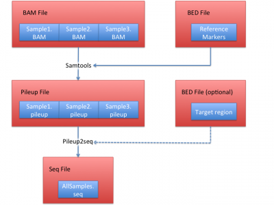
LASER Data Processing Procedure
1. Obtain pileup files from BAM files
The first step is to generate a BED file:
cat ../resource/HGDP/HGDP_938.site |awk '{if (NR > 1) {print $1, $2-1, $2;}}' > HGDP_938.bed
This BED file contains the positions of all the reference markers.
Then we use samtools to extract the sequence bases overlapping these 632,958 reference markers.
Assuming your BAM file name is NA12878.chrom22.recal.bam (our example BAM file), you can use this:
samtools mpileup -q 30 -Q 20 -f ../../LASER-resource/reference/hs37d5.fa -l HGDP_938.bed exampleBAM/NA12878.chrom22.recal.bam > NA12878.chrom22.pileup
to obtain a pileup file named NA12878.chrom22.pileup. It is required to keep the .pileup' suffix.
2. Obtain a seq file from pileup files.
After obtaining pileup files from each BAM file, you can convert them into a single seq file before running LASER.
Use the same site file and all generated pileup files from step 1 to generate a seq file:
python pileup2seq.py -m ../resource/HGDP/HGDP_938.site -o test NA12878.chrom22.pileup
You should obtain test.seq file after this step.
Estimate ancestries of sequence samples
The easiest way to perform LASER using its exemplar data is:
./laser -s pileup2seq/test.seq -g resource/HGDP/HGDP_938.geno -c resource/HGDP/HGDP_938.RefPC.coord -o test -k 2
Upon successful calculation, you will find a result file "test.SeqPC.coord".
Interpret LASER outputs
Upon successfully launching LASER command line as above, the output messages should be similar to below:
   ===================================================================
   ====       LASER: Locating Ancestry from SEquencing Reads       ====
   ====            Version 1.0 | (c) Chaolong Wang 2013            ====
   ====================================================================
   Started at: Fri Nov 15 01:05:48 2013
   938 individuals are detected in the GENO_FILE.
   632958 loci are detected in the GENO_FILE.
   1 individuals are detected in the SEQ_FILE.
   632958 loci are detected in the SEQ_FILE.
   938 individuals are detected in the COORD_FILE.
   100 PCs are detected in the COORD_FILE.
   Parameter values used in execution:
   -------------------------------------------------
   GENO_FILE (-g)resource/HGDP/HGDP_938.geno
   SEQ_FILE (-s)pileup2seq/test.seq
   COORD_FILE (-c)resource/HGDP/HGDP_938.RefPC.coord
   OUT_PREFIX (-o)test
   DIM (-k)2
   MIN_LOCI (-l)100
   SEQ_ERR (-e)0.01
   FIRST_IND (-x)1
   LAST_IND (-y)1
   REPS (-r)1
   OUTPUT_REPS (-R)0
   CHECK_FORMAT (-fmt)10
   CHECK_COVERAGE (-cov)0
   PCA_MODE (-pca)0
   -------------------------------------------------
   Fri Nov 15 01:05:50 2013
   Checking data format ...
   GENO_FILE: OK.
   SEQ_FILE: OK.
   COORD_FILE: OK.
   Fri Nov 15 01:06:01 2013
   Reading reference genotypes ...
   Fri Nov 15 01:09:15 2013
   Reading reference PCA coordinates ...
   Fri Nov 15 01:09:15 2013
   Analyzing sequence samples ...
   Results for the sequence samples are output to 'test.SeqPC.coord'.
   Finished at: Fri Nov 15 01:09:21 2013
   ====================================================================
The ancestry of input samples are store in the file test.SeqPC.coord, which content is shown below:
   popID	indivID	L1	Ci	t	PC1	PC2
   NA12878.chrom22	NA12878.chrom22	1601	0.00858193	0.977243	31.522	224.098
The ancestry coordinates for NA12878 samples are given in PC1 (31.522) and PC2 (224.098).
It is recommended to visualize this results with HGDP reference samples whose coordinates are given in file: resource/HGDP/HGDP_938.RefPC.coord
In our manuscript, an example figure is shown:
In this figure, 238 individuals were randomly selected from the total 938 HGDP samples as the testing set (colored symbols),
and the remaining 700 HGDP individuals were used as the reference panel (gray symbols).
File format
Geno file
Geno file are from reference samples. LASER use genotype of these samples as a reference panel. You can obtain geno file from VCF files using vcf2geno.
In our resource folder, we provide an example geno file for the HGDP data set (resource/HGDP/HGDP_938.geno):
Brahui	HGDP00001	1	2	1	1	0	2	0	2	1	2	2	2	1	1	2	1	0
Brahui	HGDP00003	0	0	2	0	0	2	0	2	0	2	2	2	2	0	2	2	0
Brahui	HGDP00005	0	2	2	0	0	1	0	2	1	2	2	2	2	1	2	2	1
Brahui	HGDP00007	0	2	2	0	0	2	0	2	0	2	2	2	1	1	2	2	1
Brahui	HGDP00009	0	1	0	1	0	2	0	2	0	2	2	2	2	0	2	2	0
Brahui	HGDP00011	1	1	2	1	1	2	1	1	1	2	2	2	1	1	2	2	0
Brahui	HGDP00013	1	2	2	1	1	2	1	2	0	2	2	2	2	0	2	2	0
Brahui	HGDP00015	1	1	2	0	0	2	0	2	0	2	2	2	2	0	2	2	0
Brahui	HGDP00017	1	1	2	0	0	1	0	0	0	2	0	1	1	2	2	2	0
Brahui	HGDP00019	0	2	2	0	0	1	0	1	0	2	1	2	2	1	2	2	0
The first and second columns represent the population id and individual id.
From the third column, each number represents a genotype.
To be consistent with the sequence data, genotypes should be given on the forward strand. Genotypes are coded by 0, 1, or 2, representing copies of the
reference allele at a locus in one individual.
In this geno file, we have 632,960 columns which contains 632,958 markers from column 3 to the last column.
Seq file
Seq file is generated from pileup files. It contains sequencing information and organize it in a LASER readable format.
The first two columns represent population id and individual id.
Subsequent columns are total read depths and reference base counts.
For example, column 3 and 4 are 0, 0 in the following example. That means at first marker, the sequence read depth is 0 and thus none of the reads has reference base.
We enforce tab delimiters between markers and space delimiters between each read depths and reference base counts.
On line of seq file looks like below:
NA12878.chrom22 NA12878.chrom22 0 0 0 0 0 0 0 0 0
Pileup file
Pileup file are generated using samtools. An example pileup file is shown below:
22	17094749	A	1	c	D
22	17202602	T	1	.	D
22	17411899	A	1	.	C
22	17450515	G	2	.,	9<
22	17452966	T	1	c	5
22	17470779	C	1	,	A
22	17492203	G	1	,	B
22	17504945	C	3	,..	BCA
22	17529814	T	3	..,	CCC
The columns are chromosome, position (1-based), reference base, depth, bases and base qualities.
BED file
BED file represents genomic regions and it follows UCSC conventions:
1 752565 752566
1 768447 768448
1 1005805 1005806
1 1018703 1018704
1 1021414 1021415
The columns are: chromosome, start position (0-based) and end position (1-based).
Coord file
Coord files represent the ancestries of both reference samples and sequence samples.
An example coord file looks like below:
popID  indivID  L1    Ci        t         PC1       PC2
YRI    NA19238  1409  0.304122  0.98933   52.7634   -39.7924
CEU    NA12892  1552  0.330037  0.989709  9.82674   25.2898
CEU    NA12891  1609  0.362198  0.988082  0.439573  26.8872
CEU    NA12878  1579  0.334825  0.988677  8.83775   28.1342
YRI    NA19239  1558  0.34898   0.988302  53.9104   -39.1727
YRI    NA19240  1735  0.404142  0.990264  59.8379   -45.2765
The columns are: popID means "population ID", indivID means "individual ID", L1 means number of loci has been covered, Ci means "average coverage", t means Procrustes similarity.
PC1, PC2 means coordinates of first and second principal components. You may notice L1, Ci, and t are omitted in the coord files of reference samples. The reason is that reference samples use genotypes and do not have coverage information.
Site file
Site file is equivalent to BED file and it is used here to represent marker positions. An example site file looks like below:
CHR  POS      ID          REF  ALT
1    752566   rs3094315   G    A
1    768448   rs12562034  G    A
1    1005806  rs3934834   C    T
1    1018704  rs9442372   A    G
1    1021415  rs3737728   A    G
The site file has header line, and it contains chromosome, position(1-based), id (usually marker name), ref (reference allele) and alt (alternative allele).
Advanced options
LASER has advanced options including (1) parallel computing; (2) increase ancestry inference accuracy using repeated runs; (3) generate PCA coordiates using genotypes.
See LASER Manual for detailed information.
Contact
Comments on this wiki page or questions related to preparing input files for LASER can be sent to Xiaowei Zhan.
Comments on the LASER software or the user's manual can be sent to Chaolong Wang.
This project was directed by Gonçalo Abecasis and Sebastian Zöllner at the University of Michigan.


